Queries Manager

The Query Manager is a module designed for performing advanced searches based on nodes using the graphical interface. The search criteria can range from properties to relationships.

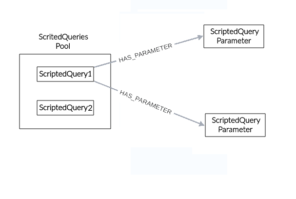
Figure 1 illustrates the module's structure. In the application, queries are stored and organized into Pools through the CHILD_OF_SPECIAL relationship, the Pools are groups of similar objects in this case, queries and can contain one or more elements. These queries, written as Groovy scripts, facilitate low-level queries within the application. Each query may include parameters that allow necessary values to be sent in the queries. The parameters are associated with the query through the HAS_PARAMETER relationship, indicating that the query has been assigned a parameter and will require it at the time of execution.

Figure 1. Queries manager Structure

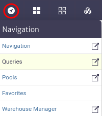
This module is part of the Navigation category, as shown in Figure 2.

Figure 2. Queries manager module

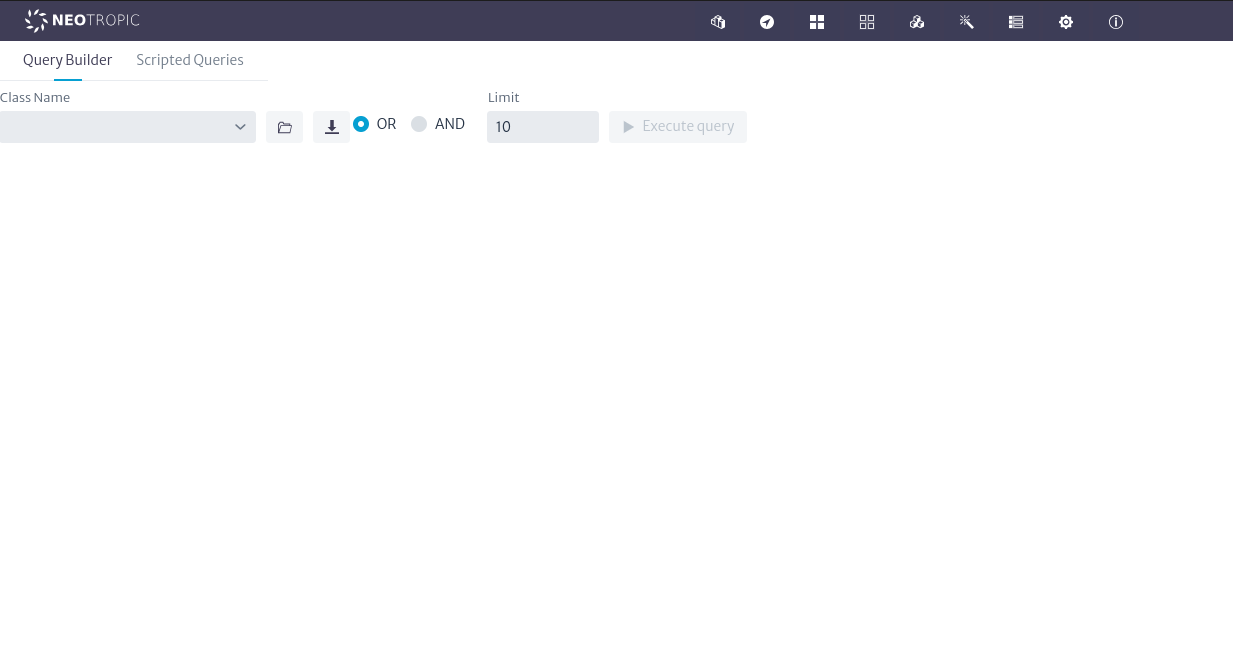
Once opened, we will see the main window of the module, as shown in Figure 3. From here you can create your queries and scripts to make queries.

Figure 3. Queries manager main window

The module allows us to perform queries in two ways: by creating a query through the graphical interface in Query Builder or through scripts in Scripted Queries.

Using Query builder

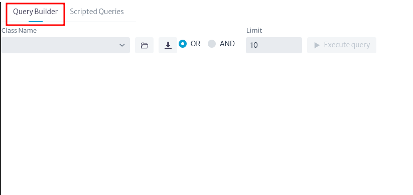
This option allows us to create queries using the module's graphical interface. To start, locate Query Builder in the main window of the module, as shown in Figure 4. This option is selected by default when entering the module.

Figure 4. Query builder

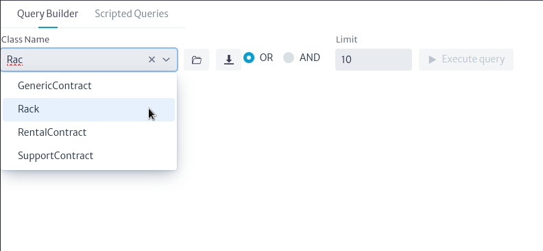
To create a query, search for and select the class of the element you want to find, as shown in Figure 5. Abstract classes are supported.

Figure 5. Select class

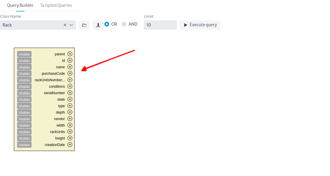
Once the class is chosen, a graphical representation of it will be placed on the canvas, as seen in Figure 6. This search box is a representation of the class node and contains each attribute of the selected class.

Figure 6. Class selected

You can search for a wider range of elements by selecting an abstract class (often called GenericSomething). In the previous example, it will search for all Racks in the database, but if you choose GenericPhysicalNode, it will search for all physical nodes, that is, all objects that can be connected via a container (see the Physical Connections chapter for more information about containers). This includes: buildings, rooms, floors, towers, shelters, and facilities.

Important

• If you want to see all objects in the database (at least all relevant to the inventory) search for InventoryObject, which is the root of all classes related to the inventory. To see the complete hierarchy see related chapter Data Model Manager

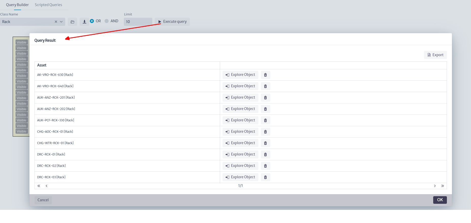
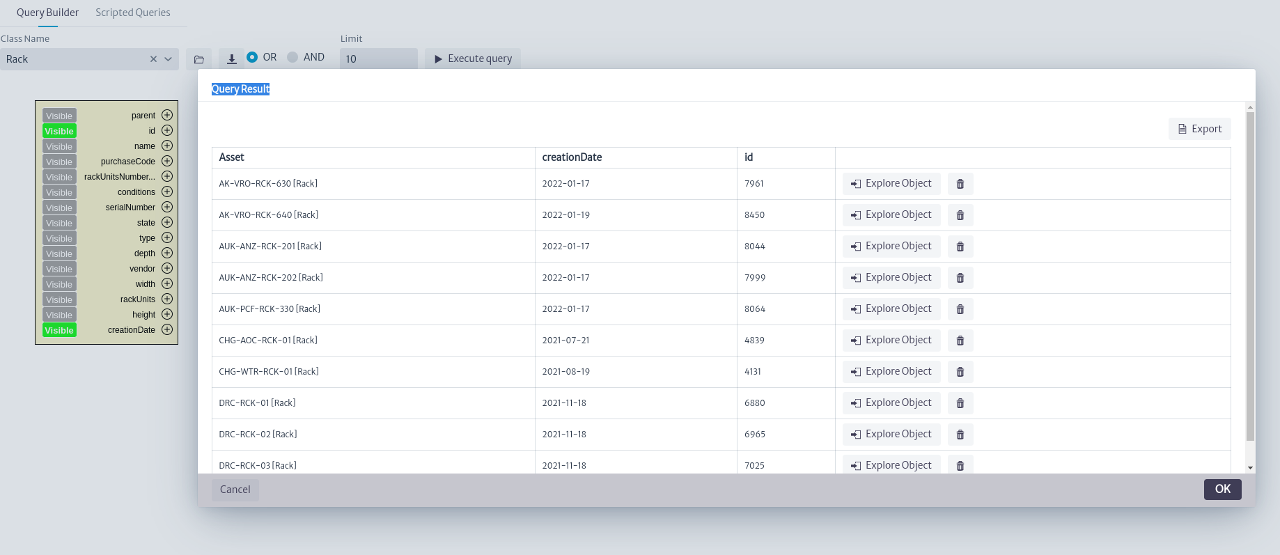
When you select a class, the Execute Query button will be enabled, allowing you to run the query. If you run it at this moment, the system will return all elements of the selected class, paginated in sets of 10 results, showing only the object's name, as seen in Figure 7.

Figure 7. Executed query

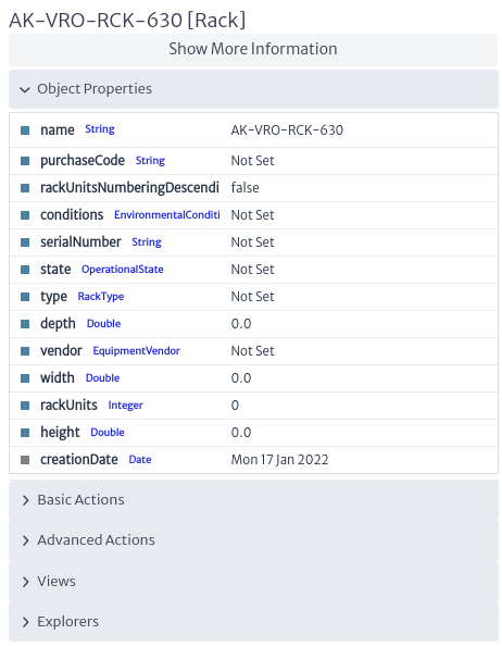
Pressing the Explore Object button will open a pop-up with the object's basic data as seen in Figure 8.

Figure 8. Object properties

Setting other attributes in the search box as visible will result in those fields being displayed in the results window, as shown in Figure 9.

Figure 9. Visible properties

Adding conditions

To perform more complex queries, you can add search conditions for any of the class attributes using the button. There are two types of attributes: those stored directly in the class node, such as name, id, creationDate, etc. Called simple attributes, and attributes whose information is stored in a separate node, called list type attributes (See list type attributes for details).

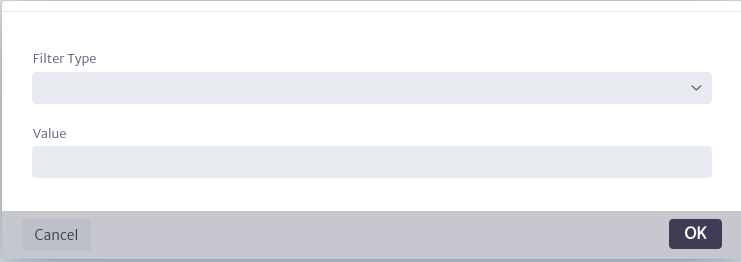
Clicking on the button for a class attribute will open the window shown in Figure 10. Enter a filter type and the desired value, then click OK.

Figure 10. Window to add attribute

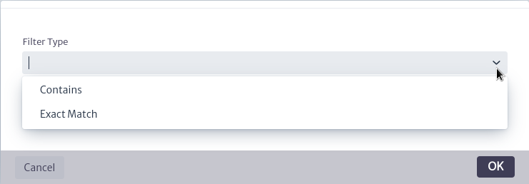
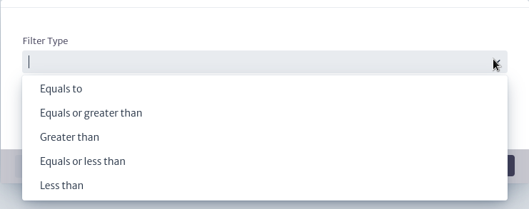
The available filter types depend on the data type of the attribute (String, Integer, etc.), as seen in the example in Figure 11 for String type attributes like name, or in Figure 12 for Integer type attributes like rackUnits.

Figure 11. Available string filters

Figure 12. Available int filters

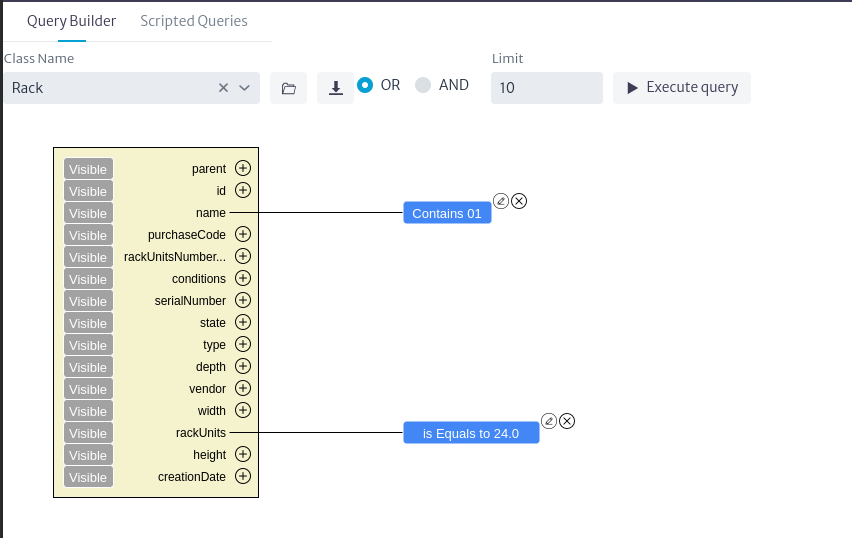
For our example, we will search for Racks in the inventory that contain "01" in their name using the Contains filter from Figure 11 on the name attribute, and that have a capacity of 24 units using the Equals to filter from Figure 12 on the rackUnits attribute. By setting these conditions for the query, you can see their graphical representation next to the corresponding attribute in the search box, as shown in Figure 13. You can edit the filters using or remove them using .

Figure 13. Filters selected

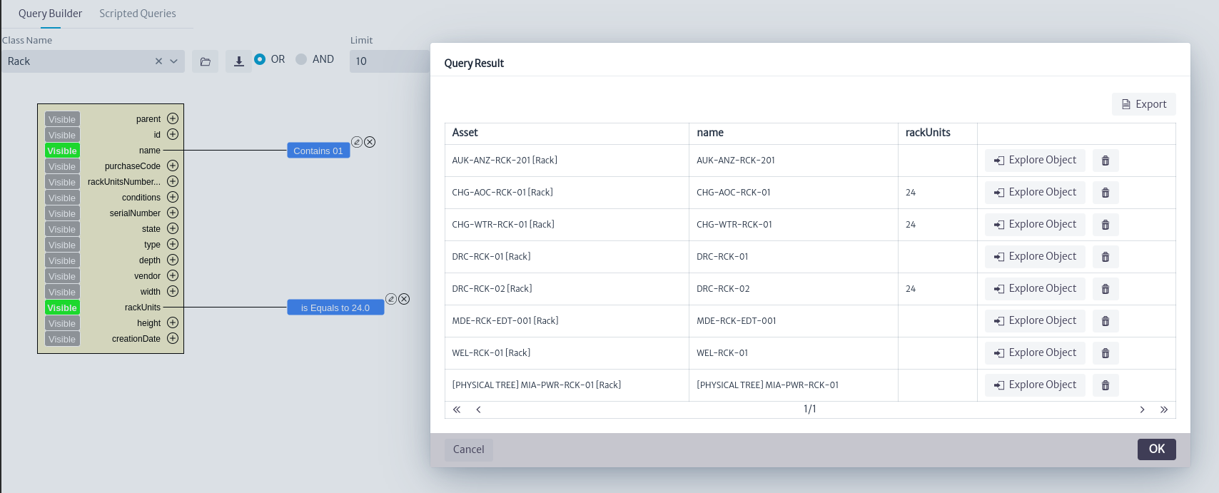
If we execute the query at this moment, we will not get the desired result as shown in Figure 14 because we need to consider how filters are applied in queries. This is similar to how it's handled in a conventional SQL statement. When we have more than two filters, we must select how they will be used in the query. We have logical operators OR and AND, which are equivalent to those used in SQL.

Figure 14. Query incomplete result

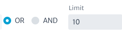
To adjust the behavior of the filters, we have the tools shown in Figure 15. From here, you can adjust the logical operator to use in the filters and the number of results the query will display.

Figure 15. Query filters

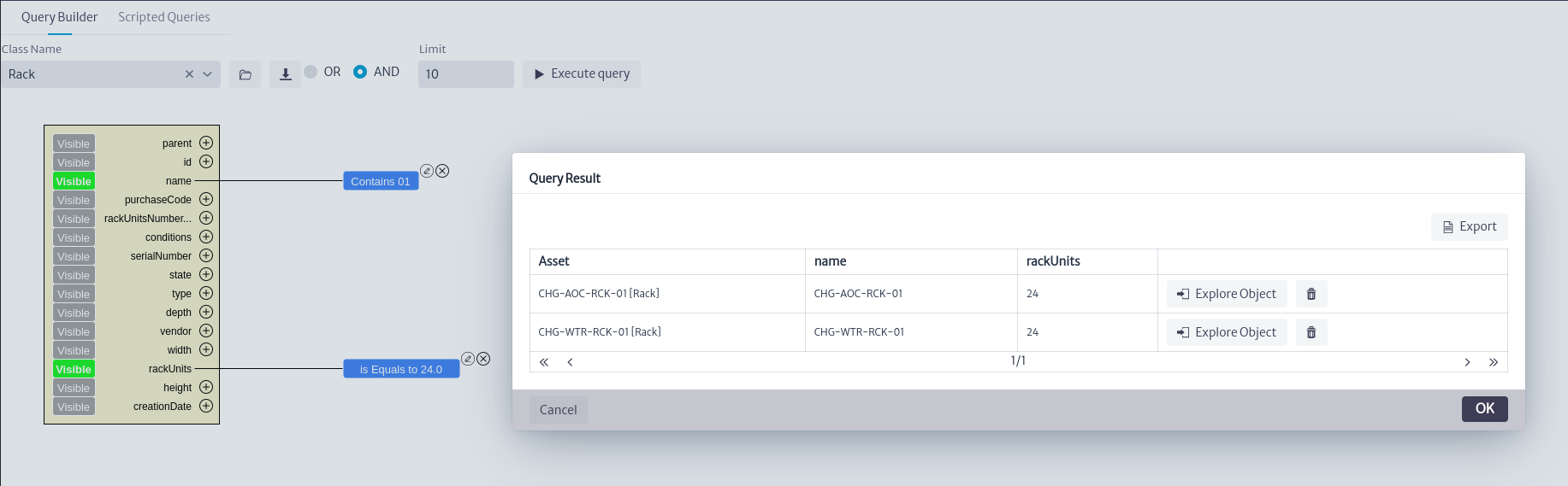
By default, the selected logical operator is OR, and the record limit is 10. In the case of our example, we select the logical operator AND and execute the query. The expected result can be seen in Figure 16.

Figure 16. Result filters

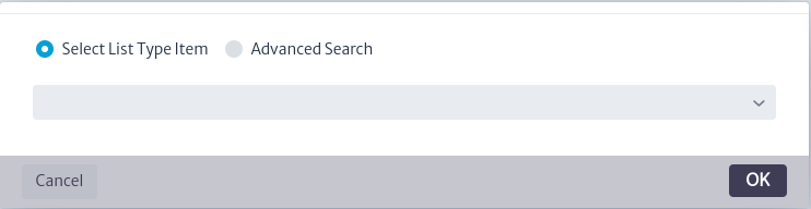
For list type attributes, when you click on the button, the window shown in Figure 17 will open. For this example, we will use the Router class, which has list attributes such as software version, model, state,vendor. We will search for routers with the vendor Huawei.

Figure 17. List type attribute filter

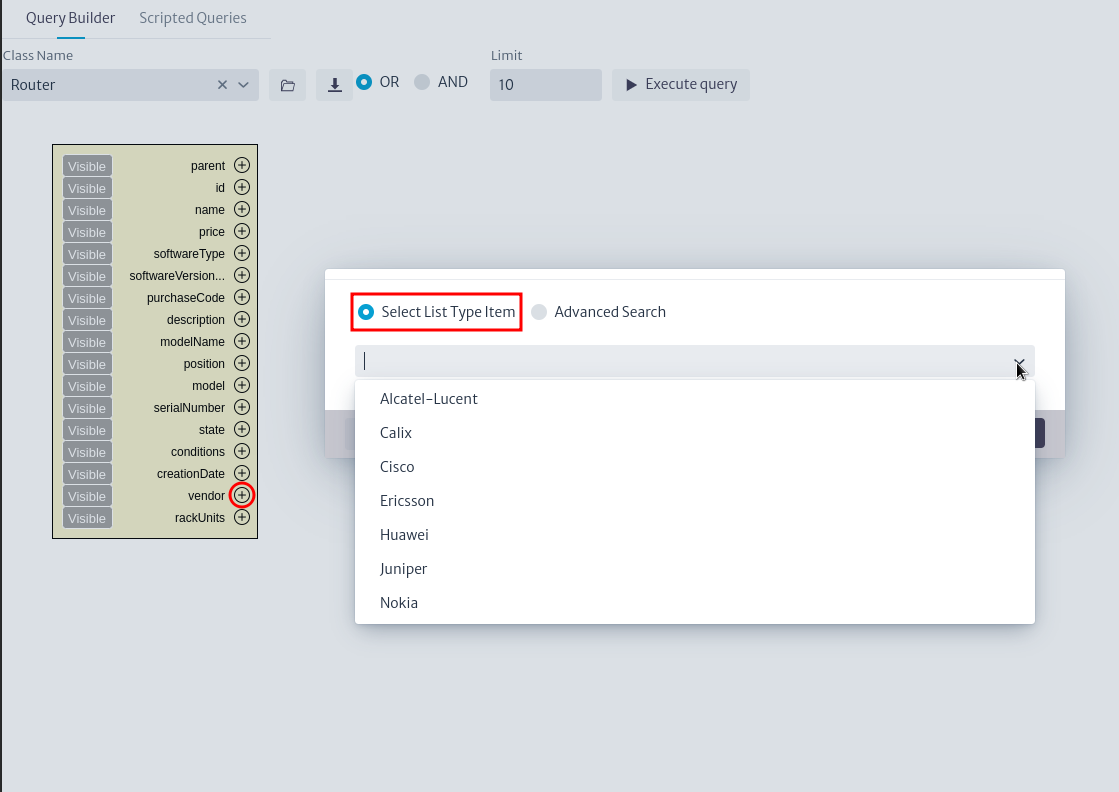
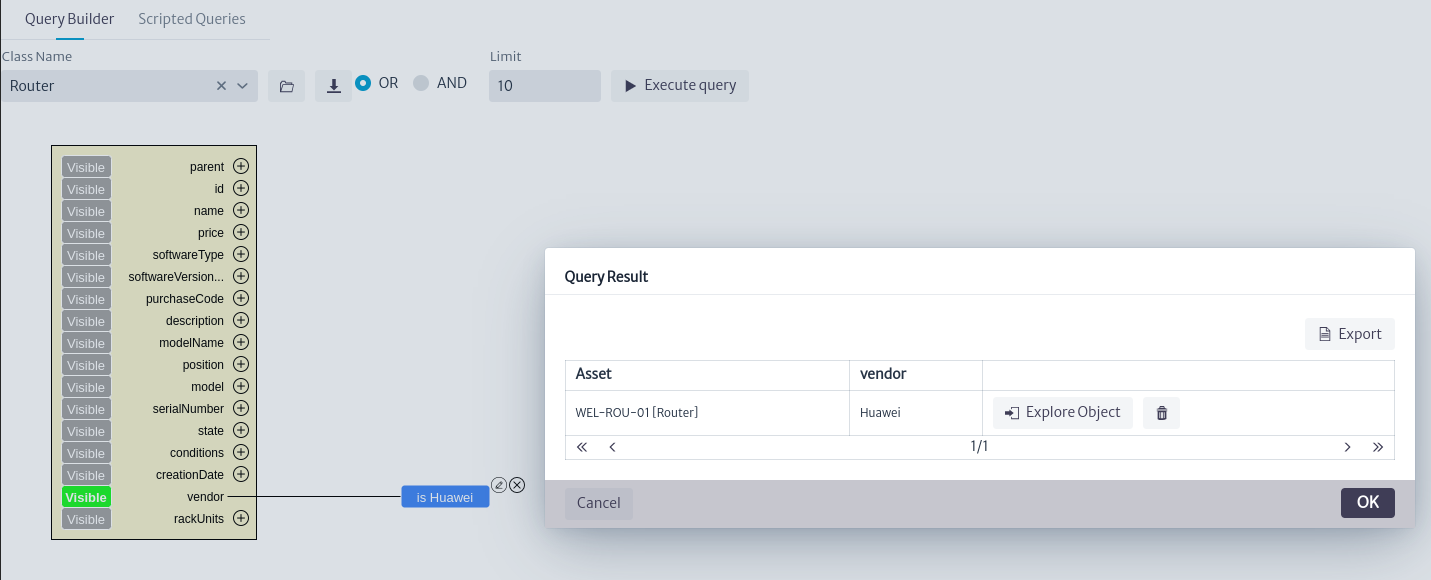
For list type attributes, we have two filter options, Select List Type Item and Advanced Search. By default, Select List Type Item is selected. In this filter, we need to choose from the attribute's list types, as shown in Figure 18. For the vendor attribute, we select Huawei, and its result can be seen in Figure 19.

Figure 18. Available list types

Figure 19. List type Search result

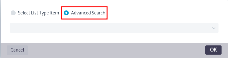
If we select the Advanced Search filter, it will not be possible to select from the attribute's list types, as shown in Figure 20. Instead, we click the OK button.

Figure 20. Advanced search window

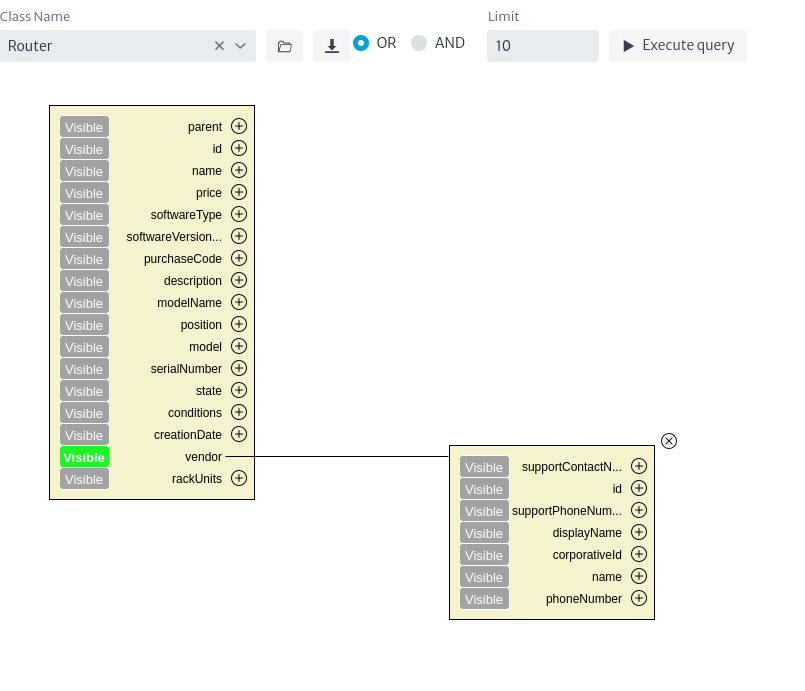
We will see that a graphical representation is immediately placed on the canvas, as shown in Figure 21. This search box represents the list type node and contains each of its attributes, similar to the search box for the selected class. As with the class, it is possible to add additional filters to the list type attributes, allowing for the creation of complex queries tailored to different scenarios.

Figure 21. Advanced search filter

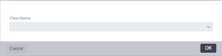
Finally, when using the button for the parent attribute, the window shown in Figure 22 will appear. This allows for a search considering the containment of the class. Refer to the containment manager for more details.

Figure 22. Select parent filter window

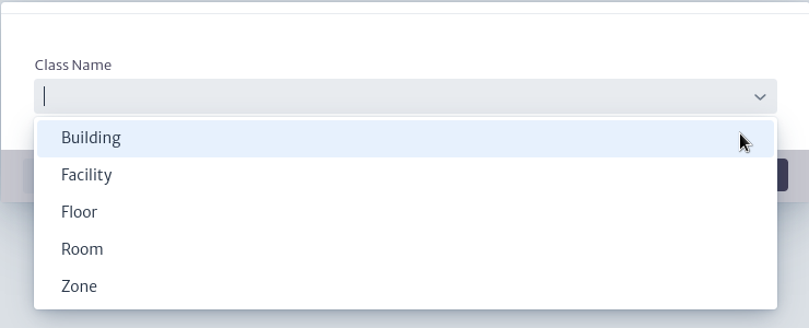
As an example, we will search for all Routers contained in the ANZ Center building, with the vendor Cisco, and whose serial number matches NZV06. To start, in the Router class, the containment classes Building, Facility, Floor, Room, and Zone are available according to its containment configuration. We choose the Building class as shown in Figure 23.

Figure 23. Select parent filter

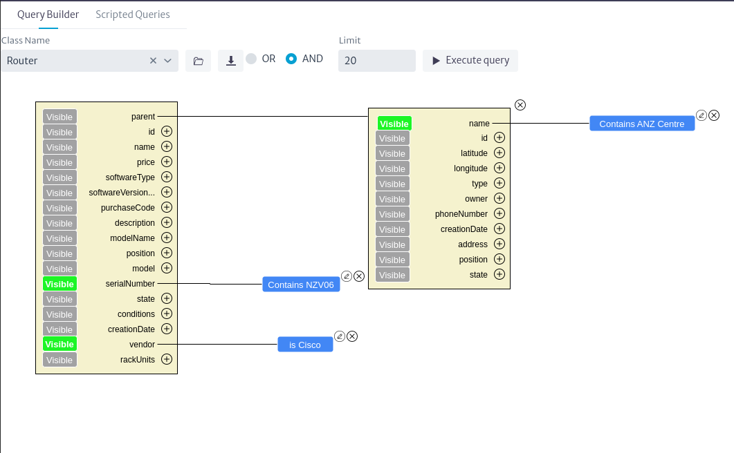
We set the filters to Contains for both the building name and serial number, with the values ANZ Center and NZV06, respectively. For the vendor, we select Cisco and choose AND as the logical connector, as shown in Figure 24.

Figure 24. Advance query

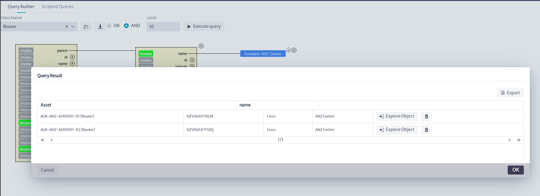
When we execute the query, we obtain the desired routers as shown in Figure 25.

Figure 25. Advance query result

Using Scripted Queries

This option allows us to create queries using Groovy scripts. The queries created with these scripts have low-level access to the application's database. Thanks to the use of scripts, it is possible to reuse these scripted queries in other modules of the application outside the queries module, allowing precise data retrieval and manipulation.

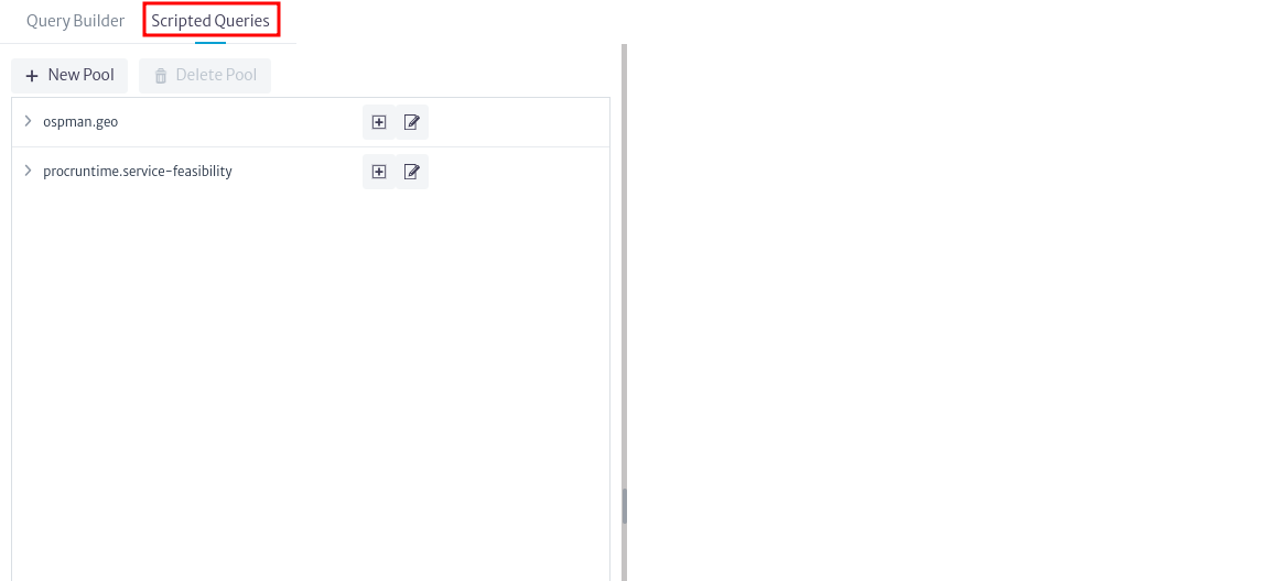
For example, the queries created in the ospman.geo pool as seen in Figure 26 are used to perform geographical queries. Refer to the Outside Plant Management for more details.

Warning The changes made by scripted queries in the database can break things if your code is wrong. Proceed with caution.

To start, locate Scripted Builder in the main window of the module, as shown in Figure 26.

Figure 26. Query builder

Manage scripted query pools

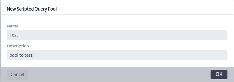
Upon entering this option, you will see the available scripts grouped into pools. To begin, create a pool using thebutton. The window shown in Figure 27 will open; enter a name, description, and click OK.

Figure 27. Add pool window

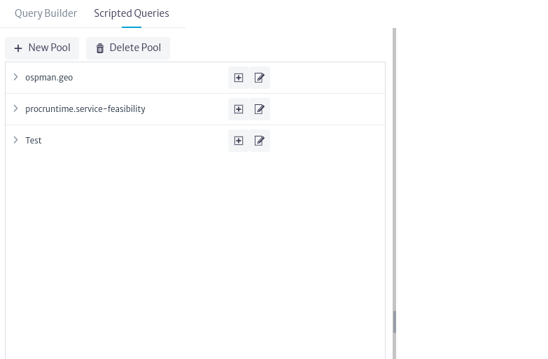
Once the pool is created, it will appear in the list of available pools, as shown in Figure 28. Conversely, if you wish to delete a pool, select it and use thebutton to delete it.

Figure 28. Pool lists

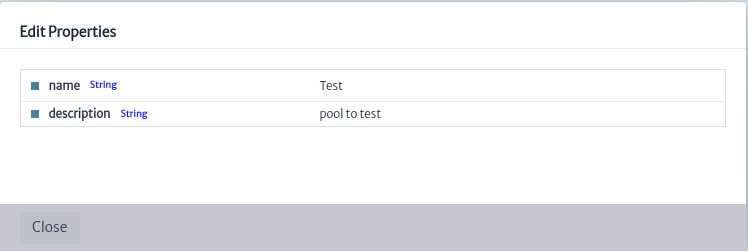
To edit the properties of a pool, use thebutton. The window shown in Figure 29 will appear, where you can edit the properties by double-clicking on the desired property.

Figure 29. Edit pool properties window

Manage scripted query

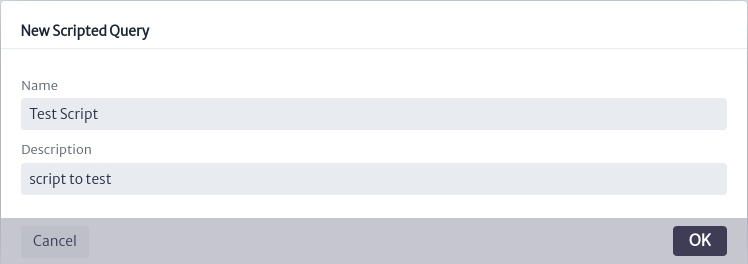
To add a script, locate the desired pool and use thebutton. This will open the window shown in Figure 30. Enter a name, description, and click OK.

Figure 30. Add script window

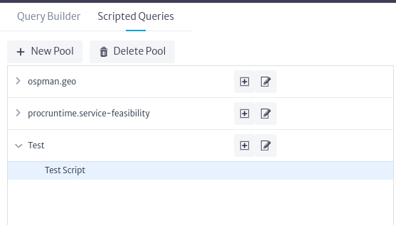
Once the script is created, use thebutton to display the scripts associated with a pool, as shown in Figure 31.

Figure 31. Scripts in pool

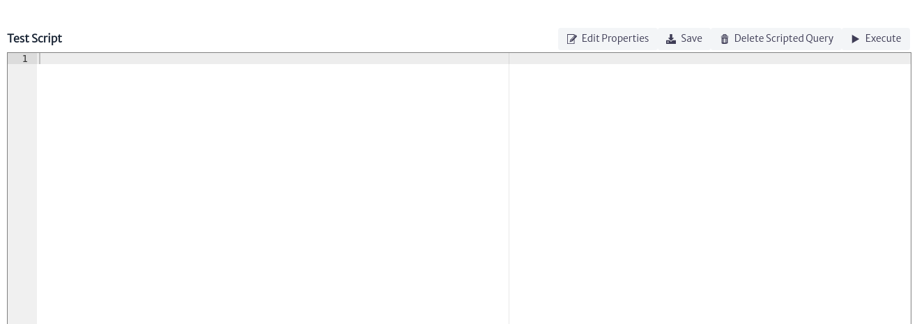
Clicking on the script will display the editor and actions associated with the script, as shown in Figure 32.

Figure 32. Script editor

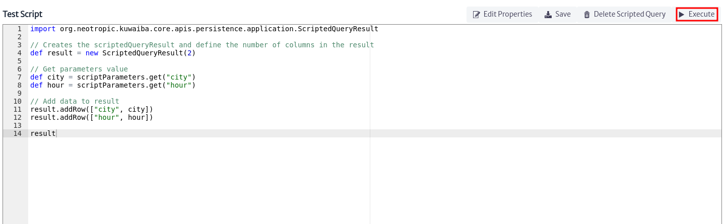
Information the creation of scripted query is beyond the scope of this document; however, you can find more detail and examples in the scripts available in this repository.

once the script is created you can save the changes using the button seen in Figure 33.

Figure 33. Script example

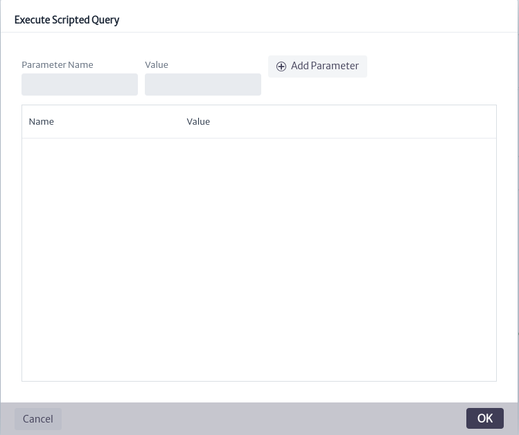
Similarly, use thebutton to save the changes to the script and open the script execution window, as shown in Figure 34.

Figure 34. Execute scripted query window

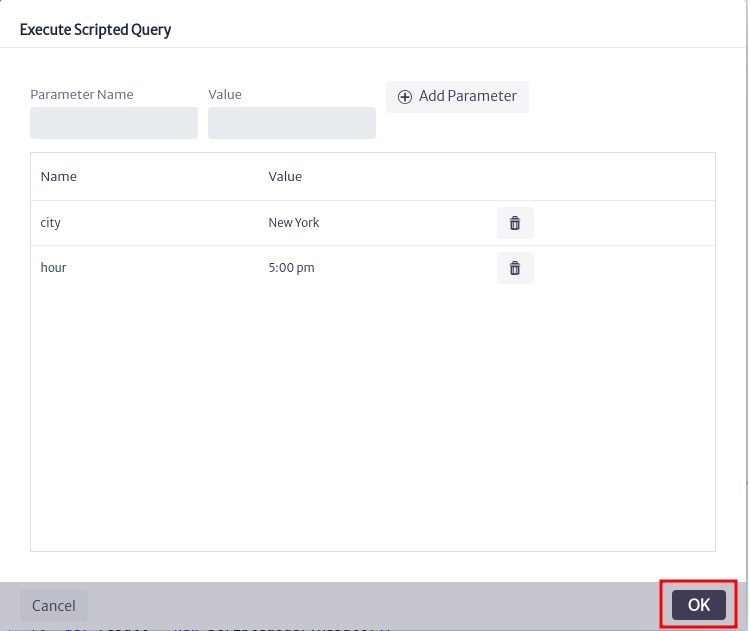
It's important to note that most scripts will require input parameters. As seen in Figure 34, you can add parameters before executing the script. To do this, enter the parameter name and value, then click . Once you've added the necessary parameters, click OK to execute the script, as shown in Figure 35.

Figure 35. Execute script

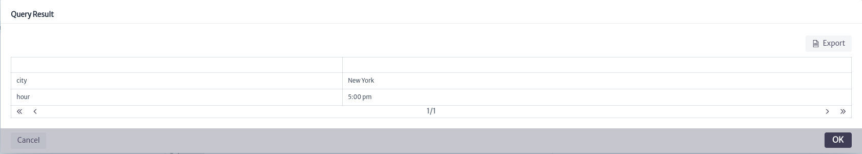
The result of the script execution will appear in the pop-up window as seen in Figure 36.

Figure 36. Script result

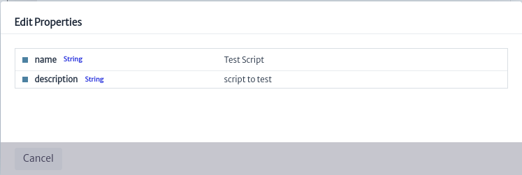
To edit the properties of a script after it has been created, use thebutton seen in Figure 33. This will open the window shown in Figure 37, where you can edit the properties by double-clicking on the desired property.

Figure 37. Edit script properties window

To delete a script, use thebutton. This will open the confirmation window shown in Figure 38. Click OK to proceed with the deletion or Cancel if you do not wish to delete it.

Figure 38. Delete script confirmation window