Outside Plant Management

The outside plant module manages the OSP views which are composed of nodes and connections and are used to represent a network.

Figure 1. Outside plant module

In this chapter the following topics will be addressed:

• Creating an FTTH OSP view
  • Adding Nodes
  • Adding Connections
• Node Tools
• Connection Tools
• Map Tools
• OSP View Tools
• Geographical Queries
• View Content Tool
  • Filters
• Splicing Tool
• Customize the Map
  • Map Provider
  • Map Center and Zoom
  • Map Labels

Creating an FTTH OSP view

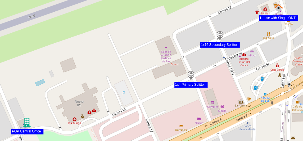
To build the osp view we are going to use as a reference the diagram in Figure 2 in which we have a central office where the OLT will be located, a primary splitter and a secondary splitter, to which the client's ONT will be connected.

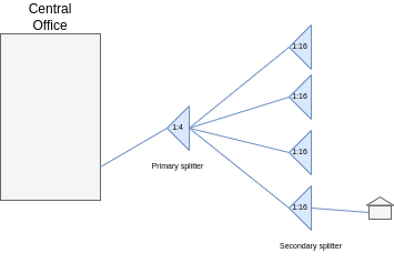Figure 2. FTTH Diagram

• Click on the create an osp view button , in the window Figure 3 enter the name and description and click on the OK button.

Figure 3. Create OSP view window

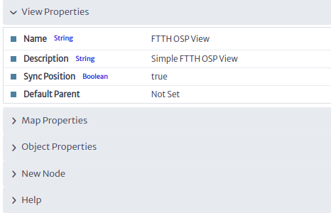
• Click on the open properties panel button to see the view properties Figure 4.

Figure 4. View properties

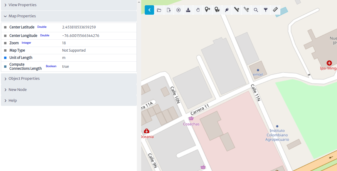
• Center the map where the network will be located. Figure 5 shows the updated map properties.

Figure 5. Map Properties

Adding Nodes

• Select the new panel node as shown in Figure 6.

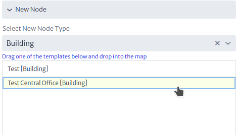Figure 6. New Node Panel

• Drag and drop to map the Test Central Office building template then the window shown in Figure 7 will appear, select the parent of the node and click the next button.

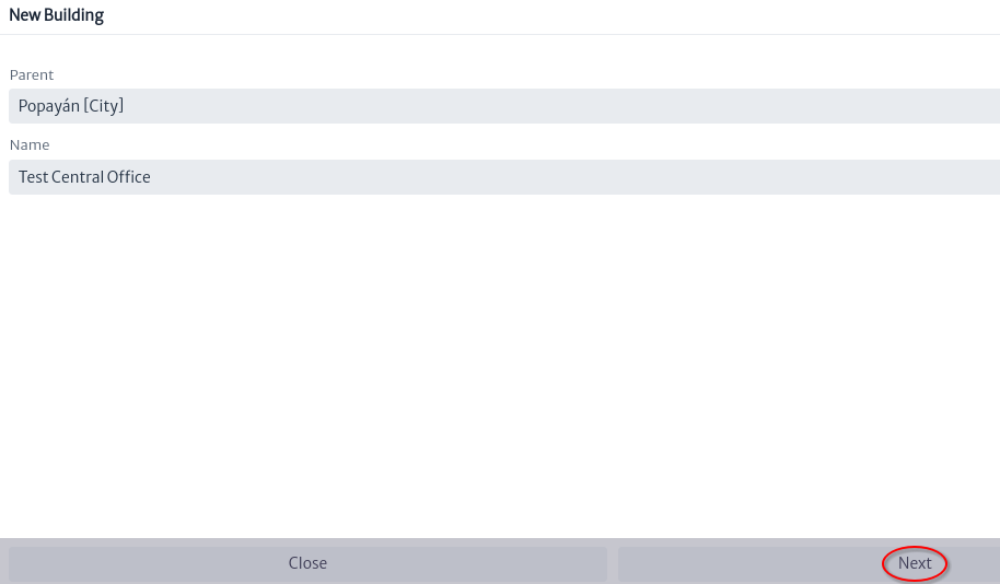Figure 7. New Building

• Using the object properties rename Test Central Office as POP Central Office Figure 8.

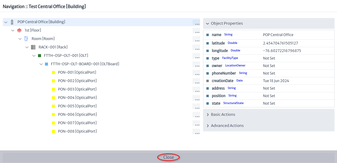Figure 8. Navigation Central Office

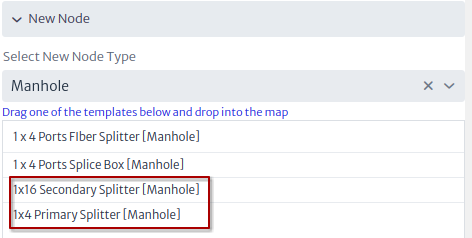
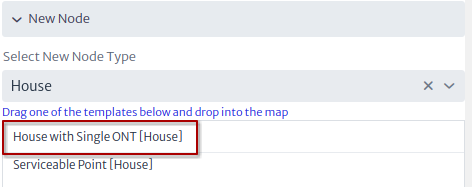
• The two previous steps are repeated to add the first and second level splitters Figure 9, and to add a house Figure 10.

Figure 9. New splitters

Figure 10. New house

The OSP view should be similar to that shown in Figure 11.

Figure 11. OSP view nodes only

Adding Connections

Once the view nodes are created, they are connected using the connection tools.

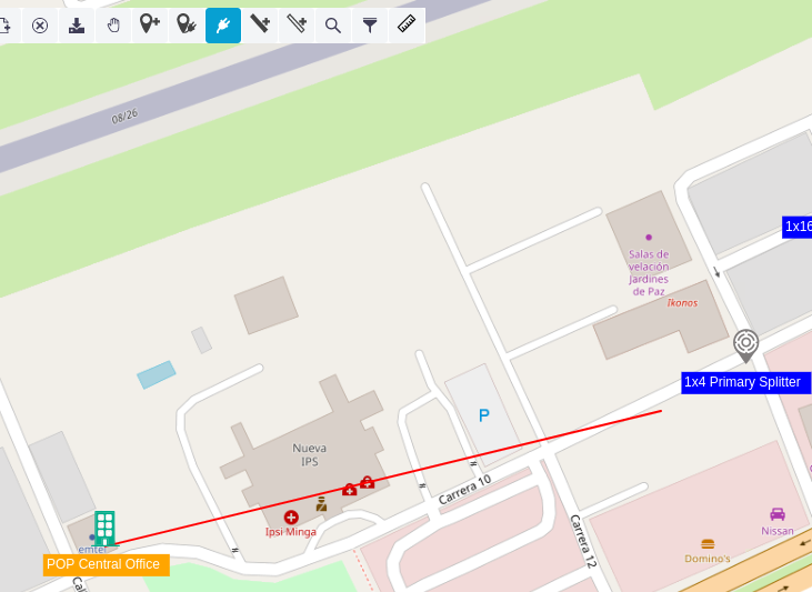
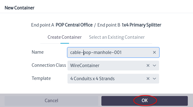
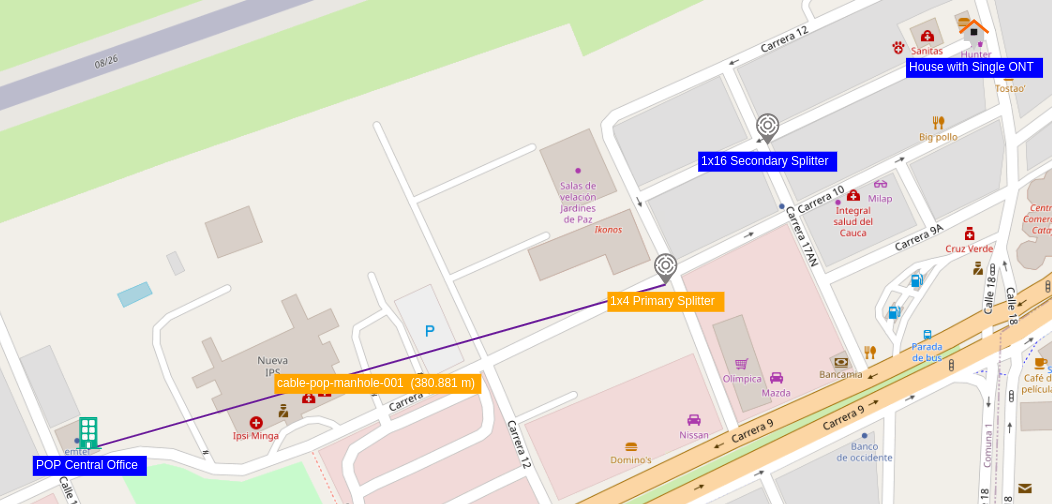
• Selecting the connection tool creates a cable between the POP Central Office and the manhole that contains the 1x4 Primary Splitter Figure 12. Then a window will appear to define the name and type of the new cable Figure 13. Click on the OK button

Figure 12. New cable

Figure 13. New container window

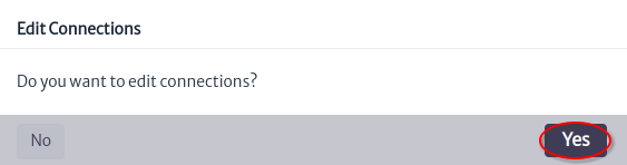
• In the window that asks whether to edit connections, click the Yes button Figure 14.

Figure 14. Do you want edit connections? window

• A window will appear to edit the connections, it will be used to create the connection between the OLT port and the primary splitter as shown in Figure 15.

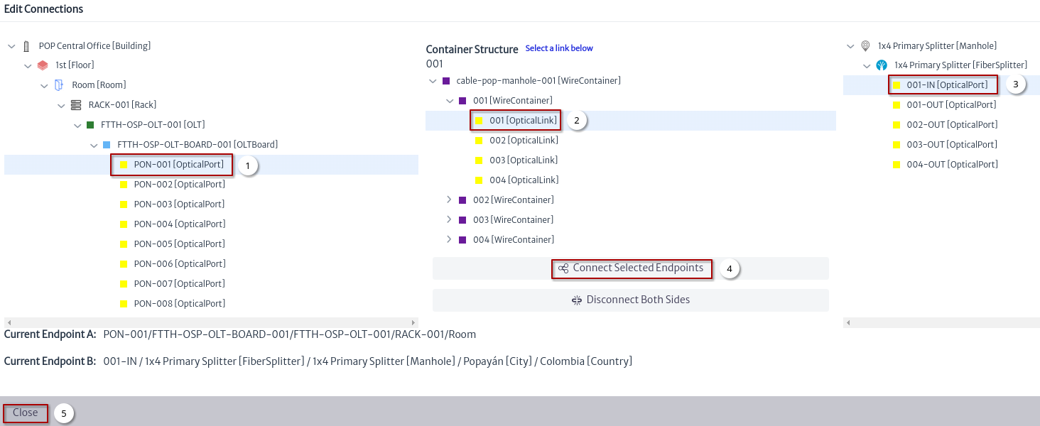Figure 15. Edit connections window

1. Select OLT port.
2. Select fiber.
3. Select IN port in primary splitter.
4. Click the button Connect Selected Endpoints.
5. Close edit connection window.

• Once the connections have been edited the OSP view looks as shown in Figure 16

Figure 16. OSP view with one connection

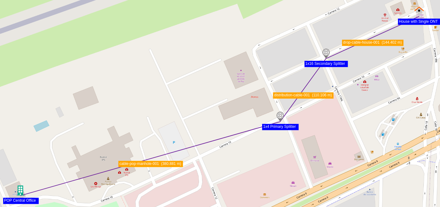
• Repeat the steps to create the connection between the primary splitter and the secondary splitter, and between the secondary splitter and the house Figure 17.

Figure 17. Simple OSP View

For more details on the connections edition see Edit Connections.

Node Tools

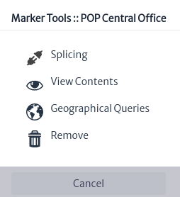
Figure 19. Node tools

Figure 19 shows the node tools window that appears when you right click on a node.

Tool	Description
	This tool is used to do fiber optic splicing of the cables that reach the selected node. See splicing tool
	Used to view the devices within the node, you can list all or use filters. See view content tool
	Using the node coordinates, geographical queries filter the network elements within a search radius.
	Remove the node from the view only, to remove the node from the inventory it is necessary to do so from the navigation module

Connection Tools

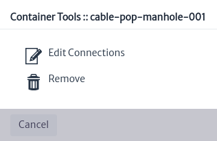
Figure 20. Connections tools

Figure 20 shows the connection tools window that appears when you right click on a connection.

Tool	Description
	The edit connection tool was covered in the adding connections section Figure 15.
	Remove the node from the view only, to remove the node from the inventory it is necessary to do so through the navigation module

Map Tools

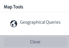
Figure 18. Map tools

Figure 18 shows the map tools window that appears when you right click on map.

Tool	Description
	Using the coordinates where you right clicked on the map, geographical queries filter the network elements within a search radius.

OSP View Tools

Figure 19. Osp View tools

Figure 19 shows the tools to manage the OSP views.

Tool	Description	Keyboard Shortcut
	Open properties panel
	Open an existing OSP View	Alt-O
	Create an OSP View	Alt-N
	Delete OSP View	Alt-D
	Save OSP View	Alt-U
	Select a node or connection	Alt-H
	Add node	Alt-M
	Add connections between two nodes using the existing containers
	Connect two nodes using a container	Alt-E
	Run a container through a single or multiple containers	Alt-C
	Run a link through a single or multiple containers	Alt-L
	Searches for a node or connection within the view	Alt-S
	Filter the nodes by class	Alt-F
	Measure distance

Geographical Queries

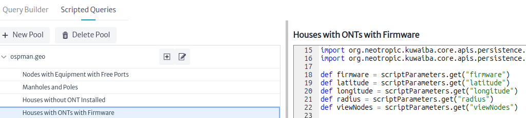
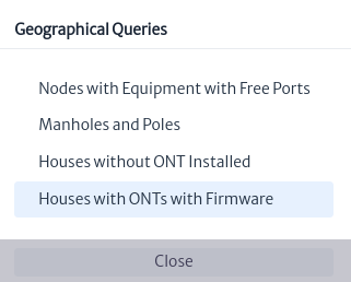
A geographic query is a scripted query from the ospman.geo pool Figure 20, this query must have the parameters latitude, longitude, viewNodes and radius plus other additional parameters that the query may require.

Figure 20. Geographical Query Pool

The latitude, longitude and viewNodes parameters are set when the query is selected Figure 21. If the action was launched from a node (see Node Tools) the latitude and longitude will be equal to that of the node. But if the action is launched from the map (see Map Tools) the values ​​are set by calculating the latitude and longitude where the right click was made. The viewNodes parameter is the list of nodes in the view.

Figure 21. Geographical Queries

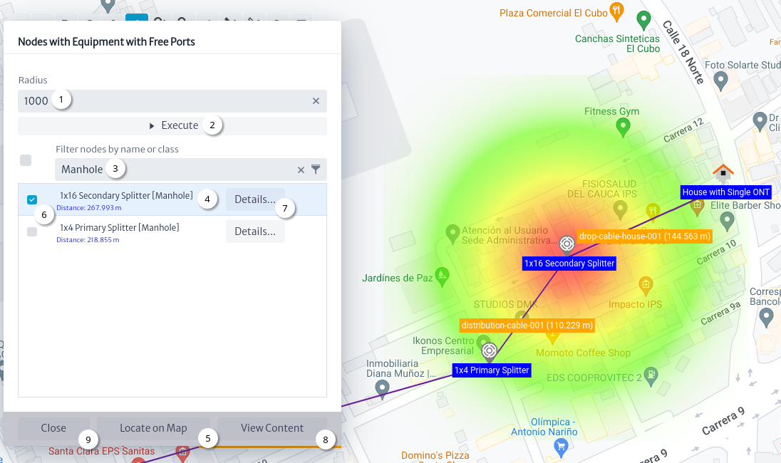
The radius parameter is a positive number in meters of a circle with center in latitude and longitude, and must be set by the user before executing the query Figure 22 as well as the additional parameters to those already mentioned.

Note

The Outside Plant module lists and executes the scripted queries Figure 21 created in the Queries module Figure 20

Figure 22. Geographical Query

Figure 22 shows the flow to execute a geographic query:

1. Set the radius in meters and other parameters if they exist.
2. Click on the Execute button.
3. Filter nodes by name or class name.
4. Select the node.
5. Click on the Locate on Map button to center the view on the selected node.
6. Check nodes to create a heat map.
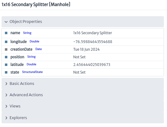
7. Click the Details... button to open an Object Options Panel Figure 23.
8. Click on the View Content button.
9. Click the Close button.

Figure 23. 1x16 Secondary Splitter details

View Content Tool

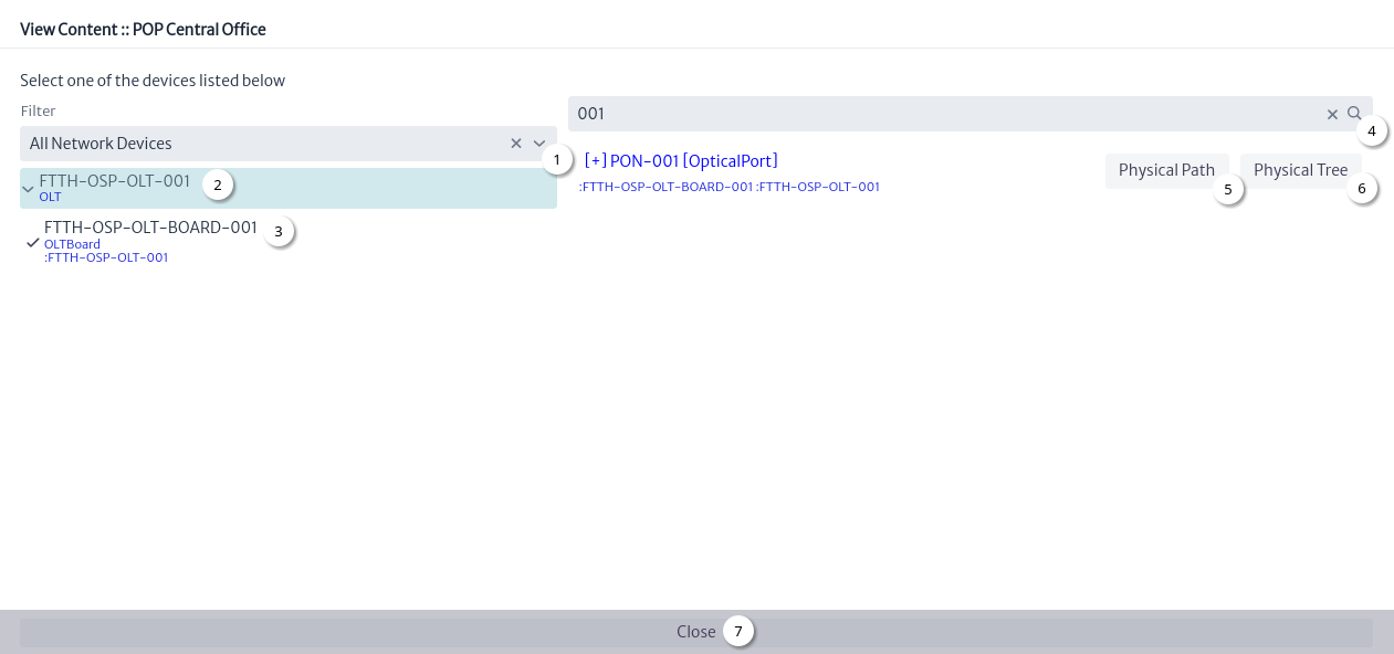
The view content tool helps you navigate the children of devices and physical connections Figure 24.

Figure 24. View content window

1. Select filter. See Filters.
2. Select device.
3. Select any of the children of the device that contains ports.
4. Search for a port.
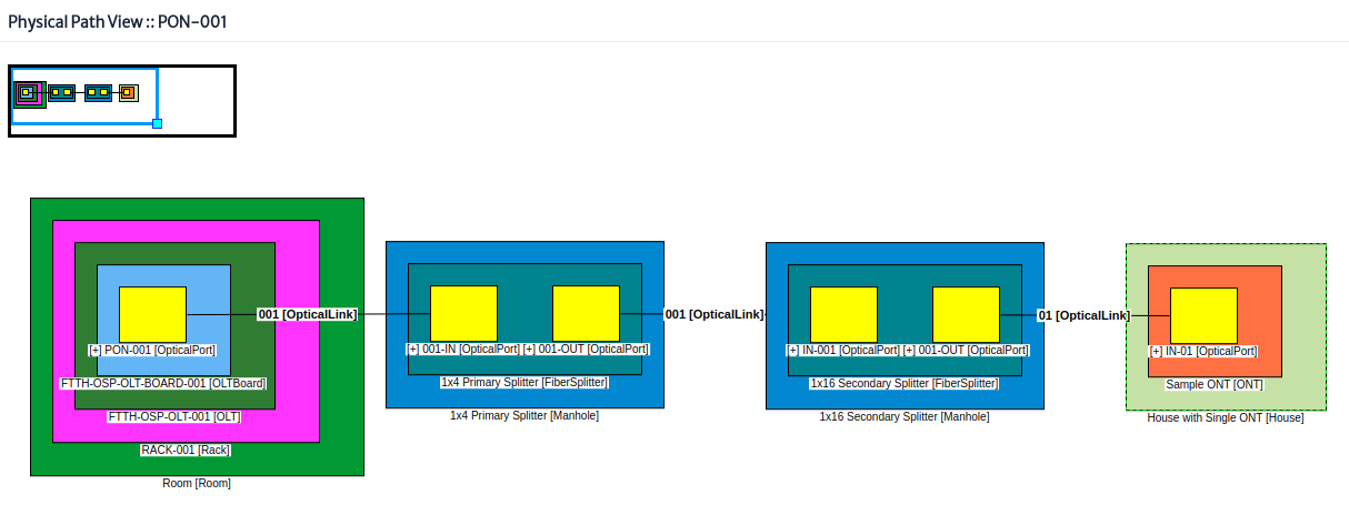
5. Click the Physical Path button Figure 25.
6. Click the Physical Tree button Figure 26.
7. Click the Close button.

Figure 25. Physical path view

For more details on the physical path view see the navigation module.

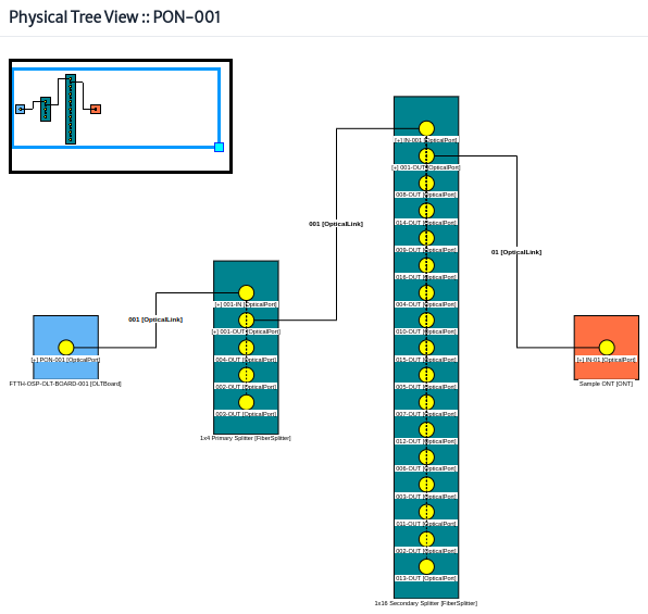Figure 26. Physical tree view

For more details on the physical tree view see the navigation module.

Filters

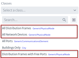
Note This is a brief introduction to filters, for more details see the Filters module.

Figure 24 shows the content of a building. The filters that appear in the filter selector are the filters defined for the Building class. Figure 27 shows the extensions for the Building class. See the data model manager.

Figure 27. Extensions for the Building class

Figure 28 shows all the filters that apply to the Building class. In general, the filters of a class are the filters of the same class and the classes that it extends.

Figure 28. Filters

Splicing Tool

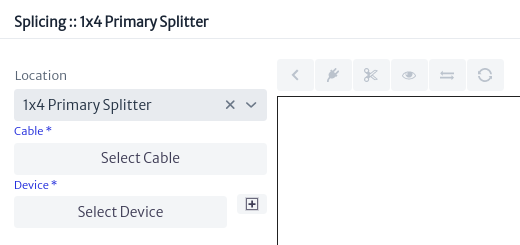
For Kuwaiba, splicing a fiber is creating the relationship endpointA or endpointB. For example using manholes that contain the primary splitter, splicing of the fibers that are not yet connected to the splitter will be done.

In Figure 29 there are three fields that must be set: the location, the cable, and a device. In the field to select the location, all the nodes in the view are listed; the value that appears by default is that of the node that opened the tool.

Figure 29. Splicing window

Click on the Select Cable button, Figure 29, a window will open that lists the cables that enter and leave the node, select the cable and then one of the tubes on which the splice will be made Figure 30.

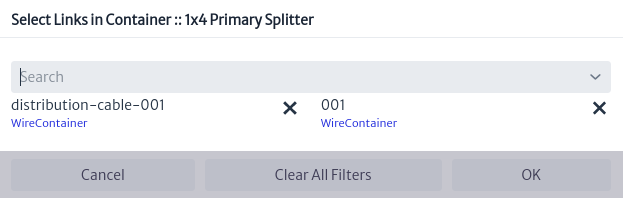Figure 30. Select cable

Click on the Select Device button, Figure 29, a window appears and will list the devices in the node, select the device on which the splice will be made Figure 31.

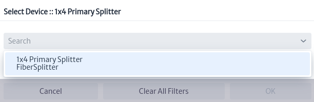Figure 31. Select device

Once the cable and device are selected, the location view is loaded Figure 32.

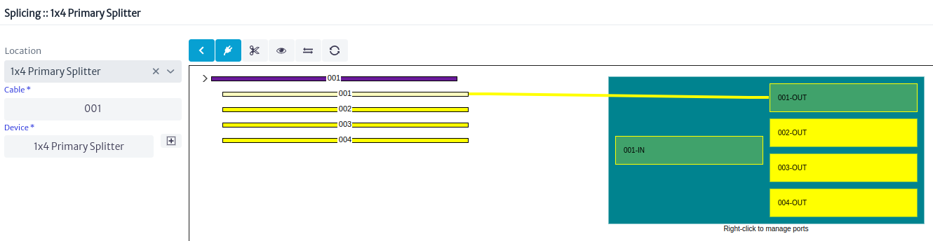Figure 32. Location view

The location of the device can be changed using the button Figure 33

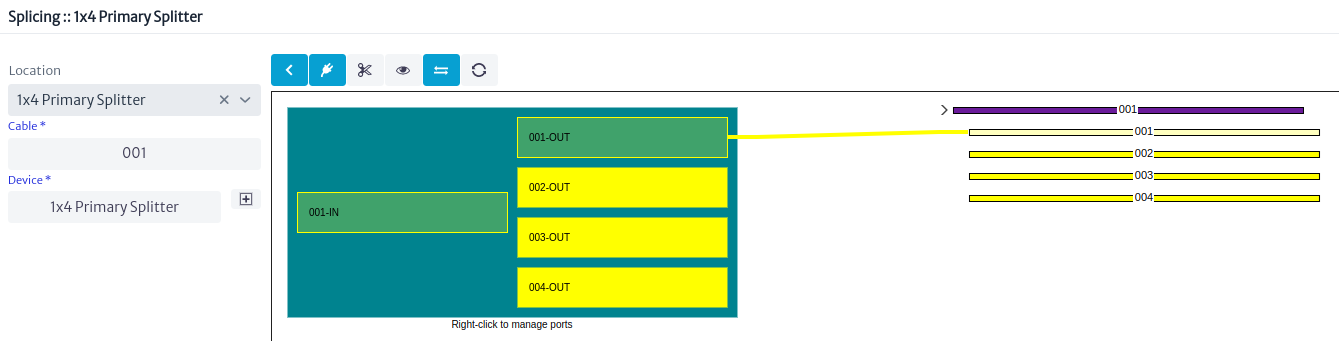Figure 33. Changed location view

The location view have some tools for management to access them, right click on the port or fiber.

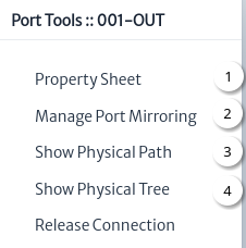
Figure 34 shows the port tools, most of them have already been explained in other chapters, the links are listed below:

Figure 34. Port tools

1. Property Sheet.
2. Manage Port Mirroring.
3. Show Physical Path.
4. Show Physical Tree.

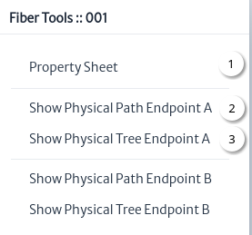
Figure 35 shows the fiber tools, all have been covered in other chapters, the list of links is shown below:

Figure 35. Fiber tools

1. Property Sheet.
2. Show Physical Path Endpoint A/B.
3. Show Physical Tree Endpoint A/B.

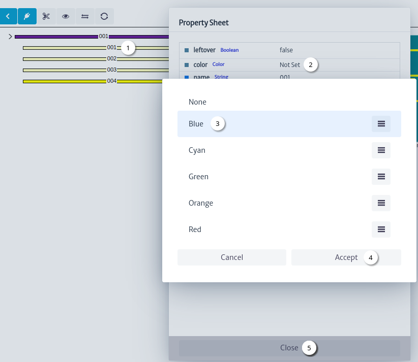
Figure 36 shows an example of using the fiber property sheet tool to set its color.

Figure 36. Set fiber color

1. Right click on the fiber, click on the property sheet tool.
2. Double click on the value of the color property.
3. Select fiber color.
4. Click on the Accept button.
5. Click on the Close button.

To update the fiber color in the location view click the refresh button Figure 37.

Note: following fiber optic cable color codes¹ define the colors for the other fibers.

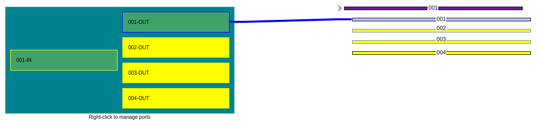Figure 37. Location view refreshed

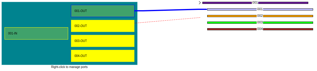
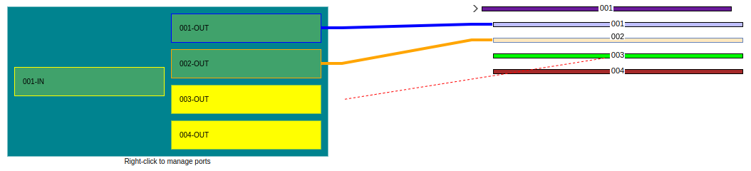
There are two ways to splice from a port to fiber Figure 38 or from fiber to port Figure 39.

Figure 38. Splicing from port to fiber

Figure 39. Splicing from fiber to port

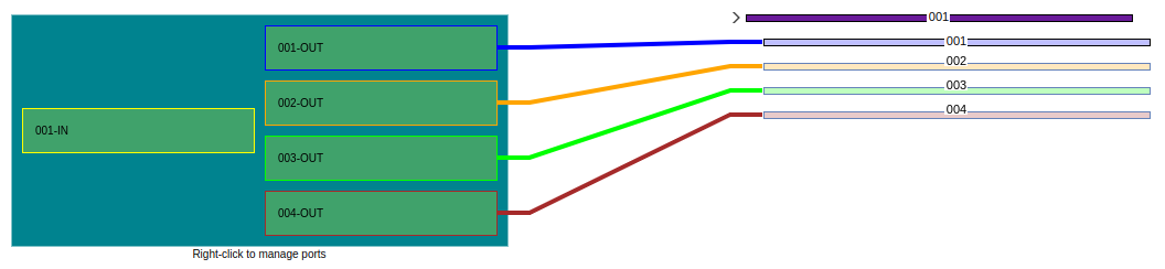
Figure 40 shows the splicing of fibers 2, 3 and 4.

Figure 40. Fiber splicing

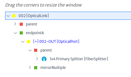
Figure 41 shows the relationships explorer for fiber 2.

Figure 41. Fiber relationships

Customize the Map

Some characteristics of the map can be changed using the configuration variables below are the changes enabled for the user.

Note: the default values ​​are listed in the configuration variables module.

Map Provider

By default the map is displayed using OpenLayers and the Open Street Map (OSM) tiled layer, to use a different map provider you must update the value of the configuration variable general.maps.provider to one of the following allowed values:

• com.neotropic.kuwaiba.modules.commercial.ospman.providers.ol.osm.OsmProvider
• com.neotropic.kuwaiba.modules.commercial.ospman.providers.ol.bmaps.BmapsProvider
• com.neotropic.kuwaiba.modules.commercial.ospman.providers.google.GoogleMapsMapProvider

Notes

• com.neotropic.kuwaiba.modules.commercial.ospman.providers.google.GoogleMapsMapProvider require the value of the configuration variable general.maps.apiKey to be set.
• com.neotropic.kuwaiba.modules.commercial.ospman.providers.ol.bmaps.BmapsProvider require the value of the configuration variables general.maps.apiKey and general.maps.provider.bmaps.imagerySet the possible values ​​of the last one are:
  • Aerial
  • AerialWithLabels
  • AerialWithLabelsOnDemand
  • Streetside
  • BirdsEye
  • BirdsEyeWithLabels
  • Road
  • CanvasDark
  • CanvasLight
  • CanvasGray

In addition to the listed providers, it is possible to extend the functionality of this module to use other providers such as Leaflet.

Map Center and Zoom

When you enter the module, the map has a center and zoom by default, this behavior can be changed by updating the configuration variables:

• widgets.simplemap.centerLatitude The default center latitude.
• widgets.simplemap.centerLongitude The default center longitude.
• widgets.simplemap.zoom The default map zoom.

Map Labels

To change the color or fill color of the labels of the nodes or edges, the following configuration variables are used:

• module.ospman.colorForLabels The color for the map labels.
• module.ospman.fillColorForEdgeLabels The fill color for the map edge labels.
• module.ospman.fillColorForNodeLabels The fill color for the map node labels.
• module.ospman.fillColorForSelectedEdgeLabels The fill color for the map selected edge labels.
• module.ospman.fillColorForSelectedNodeLabels The fill color for the map selected node labels.
• module.ospman.fontSizeForLabels The font size for the map labels.
• module.ospman.minZoomForLabels The minimum zoom level for the map when displaying.